Tuesday, June 22, 2021

3D Convolution Neural Network Using PyTorch


convolutional neural network,neural network,convolutional neural networks,convolution neural network,convolutional neural network tutorial,convolutional network,convolution neural network tutorial,convolutional neural network python,convolutional neural network stanford,pooling layer in a convolution neural network,neural networks,convolutional neural network algorithm,convolutional neural network example,convolutional neural network tensorflow,convolutional neural network andrew ng


Deep neural networks are artificial intelligence systems that excite the brain. A complex graph is used to model it, and it has at least three layers: input layer, hidden layer, and output layer. The input layer correlates to the input data's properties, while the output layer reflects the task's outcomes. Deep neuron networks come in a variety of shapes and sizes, with the Convolution Neuron Network (CNN or ConvNet) being the most suitable for image analysis

The convolution neural network (CNN) is a deep learning architecture that extracts semantic information from input data, and it represents a significant leap in computer vision. The machine can now execute visual analysis like a human owing to this architecture. The system can now recognize things in a photo or video. Object detection, face recognition, segmentation, and classification have all been made possible thanks to the combination of computer vision and deep learning.


when we talk about convolution neuron networks, most people immediately think of a 2D CNN that takes a 2D image as input. However, 3D CNN has shown to be effective in the analysis of 3D images.

If you wanted to know the difference between 2D and 3D CNN, which one is the most accurate?, and what type of activation function should I use with 3D CNN?
This article is dedicated to you!!! Let's get this party started!!


3D convolution neural network


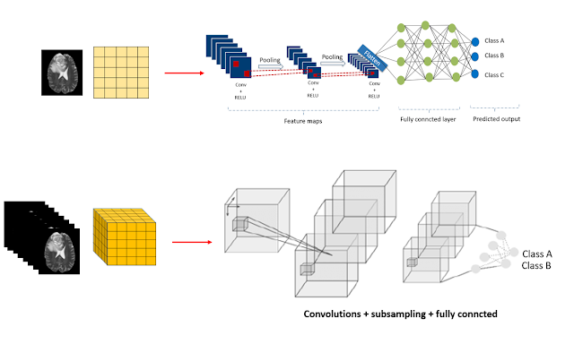
A 3D convolution neural network is a convolution neural network that can deal with 3D input data. Its structure is identical to 2D CNN,  but it takes more memory space and run time than 2D CNN due to 3D convolutions. On the other hand, it can give precise results as 2D CNN thanks to the rich input data.

neural network,convolutional neural networks,convolutional neural network,artificial neural network,deep neural network,convolutional neural network tutorial,neural networks,convolutional nerual network,convolution,convolution neural network,convolution neural network tutorial,3d convolutional neural network,temporal convolutional neural network,convolutional neural network explained,convolutional neural network python,convolutional neural network tensorflow

Note: CNN architectures include resnet, LeNet, and Densenet, among others. These architectures are also available in three-dimensional form.


3D Convolution layer :

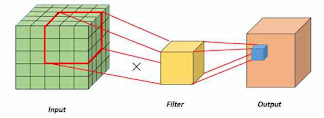
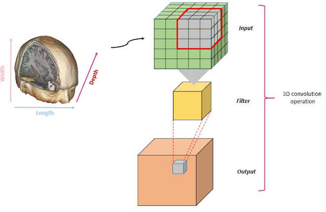
The convolution layer employs the convolution product in order to retrieve the characteristics included in the signals of the image. The output of the convolutional layer is called a feature map or activation mapAs shown in the following figure the 3d convolution operation is more sophisticated than the 2d convolution process. Requires more space and running time.


convolution,convolutional neural network,convolutional neural networks,convolutional neural network tutorial,convolutional neural network explained,convolution neural network,convolutional network,convolutional networks,animation of convolution,convolutional neural network python,feature extraction in convolution,kernel convolution,convolutions,how to convolution,transpose convolution,convolutional,deconvolution,strided convolution,convolutional layer,one by one convolutions
3D convolution operation
convolution,2d convolution,convolution operation,convolutional neural network,convolutional neural networks,animation of convolution,convolution correlation,convolution python,matrix convolution,convolution matrix,convolutions,learn convolution,how to convolution,transposed convolution,convolution matrix method,convolution matrix example,convolution basic idea,convolution neural network,convolutional neural network equations,problems on 2d linear convolution,2d linear convolution algorithm
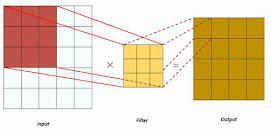
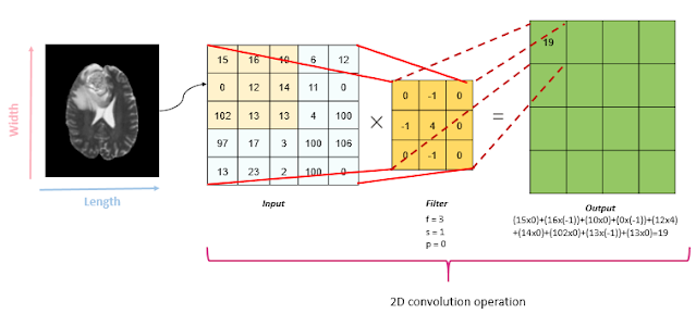
2D convolution operation


The convolution result is calculated according to a filter (f), Padding (p), and Stride (s).

  • The filter: the filter is used to analyze the image area by area.
  • The padding represents the pixels (of zero value) to add around the image in order to avoid the loss of information.
  • The stride parameter indicates the number of pixels to leap in each step to proceed in the convolution process. To know more click here!

convolution stride padding,convolution,convolution padding,convolution stride,padding in cnn,pading stride,filter,padding convolutional neural network,padding,convolutional neural network padding,stride in convolutional neural network,stride convolutional neural network,stride,convolution basic idea,tensorflow conv2d padding,keras conv2d padding,transposed convolution,convolutions,animation of convolution,convolutions over volume,padding cnn,same padding,padding deep learning,pooling layer

The convolution result is calculated in the same way as the 2d CNN. Using a three-dimensional filter.
convolutional neural network,3d convolutional neural network,3d convolution,image feature extraction using svm,image classification using svm opencv python,image classification using svm python code,convolutional neural networks,3d convolutional,image classification using svm python github,image classification using svm tensorflow,image classification using svm tensorflow 2.0,image classification,convolutional networks,image processing,convolution padding,convolution,convolution stride padding

3D Pooling layer :

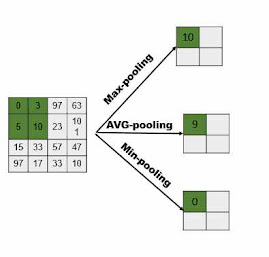
The pooling layer serves to reduce the spatial dimension of the image while keeping only the most descriptive pixels. There are 3 common methods to use: Max-pooling (select the highest value), Min-pooling (select the lowest value), Average-pooling (the average of the values).
pooling,max pooling,max pooling operation,pooling layer,global average pooling,object pooling,max pooling in cnn,what is average pooling,average pooling,what is max pooling,what is sum pooling,pooling layers,matrix operations,average pooling in cnn,how is max pooling done,pooling in unity,max pooling layer in cnn,max pooling vs average pooling,max pooling layers in cnn,pooling neural networks,global pooling in cnn,global average pooling vs max pooling,maxpooling,array initialization
2D pooling operation

pooling,pooling layers,global average pooling,object pooling,venous pooling,tooling,max pooling layers in cnn,pooling samples for testing sars-cov-2,maxpooling,inspiration,music generation,inhalation,optimization,inflammation,feminisation,dna isolation,rna isolation,convolution padding,3d information,feminization surgery,education,animation,inception,graph convolution,shape segmentation,interventional cardiology,convolution stride padding,preparation of lysis buffer,educational,convolution


Code : 

3D Fully connected layer 

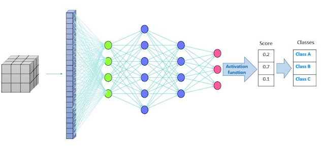
The fully connected layer applies to a previously flattened input. It connects each neuron in one layer to all neurons in the other layer, it works like the multi-perceptron neural network. In the case of classification, the result of this layer is a vector that contains the probability values ​​of the classification.
image classification,classification,deep learning image classification,python image classification,image classification alogrithms,3d cnn in keras,convolutional neural network tensorflow example,neural nets example,3d convolution neural network,multi layer perceptron,3d convolution,fc layer,what is cnn in deep learning,what is cnn in machine learning,pooling layers,dense layer,3d deep learning,zero padding in cnn,cnn in deep learning,cnn in python,cnn in arabic,padding in cnn

Code : 
 

 import torch.nn as nn
import torch.nn.functional as F

fullyC1 = nn.Linear(INsize, OUTsize) 

Note: We may also provide bias (True (meaning learn additive bias) or False), device, and dtype as parameters.

Activation functions

The activation function is a mathematical function that considers the weight and bias to determine which outcome will be transferred to the next neuron. There are several activation functions that can be classified into linear and non-linear activation functions. The choice of such an activation function depends on the type of problem to be solved.
Note: The activation functions used in 2D CNN  are also used in  3D CNN.

Linear activation functions

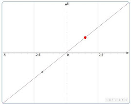
The curve is linear where the function is f(x)=y, as indicated in the figure.

activation functions,activation function,sigmoid activation function,relu activation function,softmax activation function,tanh activation function python,types of activation function in neural network,linear activation function,tanh activation function,activation function in neural network ppt,different types of activation functions in neural networks,activation function relu,step activation function,linear activation functions,leaky relu activation function

Drawback: They are incapable of dealing with complex problems.

Non-linear activation functions

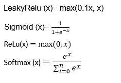
These functions are the most used, they are efficient in complex problems compared to linear functions. Sigmoid, ReLU (Rectified Linear Unit), and softmax are examples of nonlinear functions.
activation function,activation functions,sigmoid activation function,tanh activation function python,softmax activation function,activation function explained,activation function relu,relu activation function,activation function in neural network,relu activation function python,types of activation function in neural network,activation functions in neural networks,why is relu a non-linear activation function?,activation functions neural networks,linear function,non linear activation function, softmax

Code:

 import torch.nn as nn
import torch.nn.functional as F

conv_Pool_layer = nn.Sequential(
nn.Conv3d(in_val, out_val, kernel_size=(3, 3, 3), padding=0),
nn.LeakyReLU(),
nn.MaxPool3d((2, 2, 2))

A simple comparison of 3D CNN with 2D CNN for image classification of brain tumors


import torch.nn as nn
#LeakyReLU activation function 
AF_LeakyReLU = nn.LeakyReLU()

#Sigmoid activation function
AF_Sigmoid = nn.Sigmoid()

#Softmax activation function
AF_Softmax = nn.Softmax()

#ReLU activation function
AF_ReLU = nn.ReLU()
What are the key observations that can be made if we try to apply 3D CNN and 2D CNN in the same context? In this post, I use a simple experiment to reply to this question. On brain tumor imaging datasets, I compare the performance of 2D and 3D CNNs. 

2D and 3D CNNs were trained To classify brain tumor images into the type of tumor. The neural network's input was a brain tumor image, and the deep neural network's output was the type of tumor.
 
So, for 2D CNN, we utilized 3264 images (Brain Tumor Classification (MRI) ) and for 3D CNN, we used 461 images (Brain Tumor Segmentation dataset). There are 155 slices in each 3D image. So the first thing we can note is that the number of 2D slices in 3D images is really essential; it represents around 12 times the number of 2D slices. In this situation, a powerful computer is required to run the 3D CNN algorithm.  

image processing,image classification,segmentation of brain tumors from mri using deep learning,brain tumor detection,brain tumors images,brain tumor,image classification using svm python github,pytorch with brain tumor, pytorch,cnn,pytorch cnn,cnn using pytorch,pytorch cnn tutorial,3d cnn,pytorch3d,cnn en pytorch,3d cnn in keras,pytorch 3d,cnn useing pytorch,3d,code ann pytorch,pytorch course,convolutional ann pytorch,pytorch tutorial,tutorial pytorch,pytorch gan mnist,red neuronal en pytorch,pytorch simple gan,3d convolutional neural network,pytorch summer hack,tutorial de pytorch,pytorch sequential,pytorch original gan,3d convolution neural network


The first thing you'll notice is that training 3D CNN takes longer than training 2D CNN. To make it faster, start with a small batch or reduce the number of slices in each 3D image.

As we've seen in earlier sections, 3D CNN is thought to be more accurate than 2D CNN due to the number of slices used. However, the outcome is unexpected; the surprise is that 3DCNN produces unpredictable results.

I first noticed that after reaching a high in the learning stage of 3DCNN, the accuracy curve begins to decline. In addition, there is a significant difference between the accuracy curves in the training and testing stages. these two signals imply that there is a problem of overfitting.

Most popular frameworks


 Pytorch 


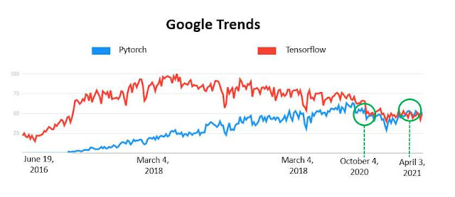
Pytorch is a deep learning framework, developed by Facebook’s AI Research lab (FAIR) in 2016, it is written in different languages like Python and C++. This framework is gaining in popularity since it is adaptable and provides the elements that make it acceptable for researchers. Thanks to the simplicity of use and efficiency, several companies replace the use of TensorFlow with PyTorch. Also, the statistics provided by google trends approve that. Among its strengths it is very object-oriented, it adapts to large datasets, faster than other frameworks, it offers the possibility of running code on GPU or CPU.
tensorflow,tensorflow vs pytorch,pytorch vs tensorflow,pytorch,keras vs tensorflow vs pytorch,pytorch vs tensorflow for nlp,pytorch vs tensorflow benchmarks,pytorch vs tensorflow for deep learning,difference between pytorch and tensorflow,pytorch vs tensorflow 2021,tensorflow tutorial,keras vs tensorflow,deep learnign with keras tensorflow and pytorch,pytorch o tensorflow,pytorch or tensorflow,pytorch vs tensorflow 2018,pytorch vs tensorflow 2019,tensorflow vs pytorch 2020

Keras 

Keras is an open-source library that is specialized in neural network tasks. It is built on multiple platforms, including TensorFlow, Theano, Toolkit

The Keras library was created by François Chollet in 2015. It is easy to use and is characterized by its low speed.

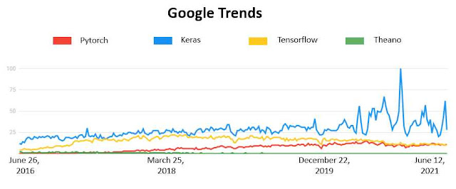
According to statistics from Google Trends, Keras has retained the first place as the most searched framework on Google since 2016.

tensorflow vs pytorch,tensorflow,pytorch vs tensorflow,keras vs tensorflow vs pytorch,keras vs tensorflow,keras vs pytorch,tensorflow vs keras,tensorflow tutorial,pytorch vs tensorflow for nlp,deep learnign with keras tensorflow and pytorch,pytorch vs tensorflow benchmarks,pytorch vs tensorflow for deep learning,pytorch vs tensorflow vs keras vs theano,theano,keras vs torch,keras,pytorch vs tensorflow vs keras,pytorch vs keras vs tensorflow,scikit learn vs tensorflow vs keras vs pytorch

Use Case

We will implement 3D CNN step by step to understand all of the theoretical information in the previous sections.
We'll go through the process of developing a classifier for 3D MNIST digits in this section.

1) Install PyTorch 

All instructions for installing this framework can be found in the video below.


2) Dataset 

In this lesson, we will use 3D Mnist, a free dataset. Before we begin, we must first generate an overview of our dataset.

This dataset is available for download on the Kaggle website.
It contains 3D images of handwritten digits. It includes ten classes (numbers:  0-9) and a training set of 10,000 images and a test set of 2000 images.

3) Implementation

3.1) Read Data

In the path variable, you should write the path to the dataset folder.

Code :  

 
import h5py 
path_dir="write here the path to the dataset folder"
with h5py.File(path_dir+"full_dataset_vectors.h5", "r") as data:    
    X_train = data["X_train"][:]    
    y_train = data["y_train"][:]   
    X_test = data["X_test"][:]     
    y_test = data["y_test"][:]

Let's have a look at the data types in the 3D Mnist dataset.

Code : 

print('X_train   :   shape:', X_train.shape, '         type:', type(X_train))
print('y_train   :   shape:', y_train.shape, '              type:', type(y_train))
print('X_test    :   shape:', X_test.shape, '          type:', type(X_test))
print('y_test    :   shape:', y_test.shape, '               type:', type(y_test))

result


3.2) Reshape data

MNIST images in 3D space are 16x16x16 size. We resize each image vector to 16x16x16, as shown below.

Code :  

 import torch
def transform_images_dataset (data):
    #Binarize_images_dataset
    th=0.2
    upper=1
    lower=0
    data = np.where(data>th, upper, lower)
    #data_transform_channels
    data = data.reshape(data.shape[0], 1, 16,16,16)
    data = np.stack((data,) * 3, axis=-1) # 
    return(torch.as_tensor(data))
X_train = transform_images_dataset(X_train)
X_test = transform_images_dataset(X_test)

def one_hit_data (target): 
    # Convert to torch Tensor
    target_tensor = torch.as_tensor(target)
    # Create one-hot encodings of labels
    one_hot = torch.nn.functional.one_hot(target_tensor, num_classes=10)
    return(one_hot)

y_train= one_hit_data (y_train) 
y_test= one_hit_data (y_test)
print('X_train   :   shape:', X_train.shape, '          type:', type(X_train))
print('y_train   :   shape:', y_train.shape, '                     type:', type(y_train))
print('X_test    :   shape:', X_test.shape, '           type:', type(X_test))
print('y_test    :   shape:', y_test.shape, '                      type:', type(y_test))
 

3D Mnist classification using Pytorch

torch.nn.functional.one_hot
This function is used to convert the data to binary variables.
Example: input   T[1,0,2] 
                output T[[0 1 0]
                                [1 0 0]
                                [0 0 1]]

3.2) 3D CNN  for Mnist Classification

We'll begin building our model after we've prepared the data. 
Step1: import libraries

Code : 

 import pandas as pd
import numpy as np
from tqdm.auto import tqdm
import os
import matplotlib.pyplot as plt
import torch
from torch.autograd import Variable
import torch.nn as nn
import torch.nn.functional as F
from torch.optim import *
from sklearn.metrics import confusion_matrix
from sklearn.metrics import ConfusionMatrixDisplay 
import seaborn as sns

Step2Create a 3D convolutional neural network model for image classification

Code :  


 class CNN_classification_model (nn.Module):
    def __init__(self):
        super(CNN_classification_model, self).__init__()
        self.model= nn.Sequential(
        
        #Conv layer 1    
        nn.Conv3d(3, 32, kernel_size=(3, 3, 3), padding=0),
        nn.ReLU(),
        nn.MaxPool3d((2, 2, 2)),   
        
        #Conv layer 2  
        nn.Conv3d(32, 64, kernel_size=(3, 3, 3), padding=0),
        nn.ReLU(),
        nn.MaxPool3d((2, 2, 2)),
               
        #Flatten
        nn.Flatten(),  
        #Linear 1
        nn.Linear(2**3*64, 128), 
        #Relu
        nn.ReLU(),
        #BatchNorm1d
        nn.BatchNorm1d(128),
        #Dropout
        nn.Dropout(p=0.15),
        #Linear 2
        nn.Linear(128, num_classes)
        )
    

    def forward(self, x):
        # Set 1
        out = self.model(x)
        return out
before starting the training step, we need to create the accuracy function.

Code :  

 def accuracyFUNCTION (predicted, targets):          
    c=0
    for i in range(len(targets)):
        if (predicted[i] == targets[i]):
            c+=1
    accuracy =  c / float(len(targets))
    print('accuracy   = ', c ,'/', len(targets))
    return(accuracy)
Step3: Training the model 

Code:

 batch_size = 100    
 # Pytorch train and test sets
 train = torch.utils.data.TensorDataset(X_train.float(),y_train.long())
 test = torch.utils.data.TensorDataset(X_test.float(),y_test.long())
 # data loader with pytorch
 train_loader = torch.utils.data.DataLoader(train, batch_size = batch_size, shuffle = False)
 test_loader = torch.utils.data.DataLoader(test, batch_size = batch_size, shuffle = False)
 # we have 10 classes
 num_classes = 10
# The number of epochs (here the number of iterations is = 5000 / we have 50 epochs a batch size is 100 / 50*100=5000)
num_epochs = 50
 # 3D model
 model = CNN_classification_model()
 #You can use the GPU by typing: model.cuda()
 print(model)
 # Loss function : Cross Entropy
 error = nn.CrossEntropyLoss()
 # Learning rate : learning_r = 0.01
 learning_r = 0.01
 # SGD optimizer
optimizer = torch.optim.SGD(model.parameters(), lr=learning_r)
#***********************************************************************training***********************************
itr = 0
loss_list = []
iteration_list = []
accuracy_list = []
for epoch in range(num_epochs):
    for i, (images, labels) in tqdm(enumerate(train_loader)):
        train = Variable(images.view(100,3,16,16,16))
        labels = Variable(labels)
        #  zero_grad : Clear gradients
        optimizer.zero_grad()
        # Forward propagation / CNN_classification_model
        outputs = model(train)
        # Calculate loss value / using cross entropy function 
        labels= labels.argmax(-1)
        loss = error(outputs, labels)
        loss.backward()
        # Update parameters using SGD optimizer 
        optimizer.step()
        
        #calculate the accuracy using test data
        itr += 1
        if itr % 50 == 0:
            # Prepare a list of correct results and a list of anticipated results.     
            listLabels=[]
            listpredicted=[]
            # test_loader
            for images, labels in test_loader:

                test = Variable(images.view(100,3,16,16,16))
                # Forward propagation
                outputs = model(test)

                # Get predictions from the maximum value
                predicted = torch.max(outputs.data, 1)[1]
                
                # used to convert the output to binary variables
                predicted= one_hit_data (predicted) 
                # Create a list of predicted data
                predlist=[]
                for i in range(len(predicted)):
                    p = int(torch.argmax(predicted[i]))
                    predlist.append(p)

                
                listLabels+=(labels.argmax(-1).tolist())
                listpredicted+=(predlist)

                
                # calculate Accuracy
            accuracy= accuracyFUNCTION(listpredicted, listLabels)
            print('Iteration: {}  Loss: {}  Accuracy: {} %'.format(itr, loss.data, accuracy))

            # store loss and accuracy. They'll be required to print the curve.
            loss_list.append(loss.data)
            accuracy_list.append(accuracy) 	

3D CNN using Pytorch
Training step

Step4: Display the accuracy curve
Code :

 sns.set()
sns.set(rc={'figure.figsize':(12,7)}, font_scale=1)
plt.plot(accuracy_list,'b')
plt.plot(loss_list,'r')

plt.rcParams['figure.figsize'] = (7, 4)
plt.xlabel("Epochs")
plt.ylabel("Accuracy")
plt.title("Training step:  Accuracy vs Loss ")
plt.legend(['Accuracy','Loss'])
plt.show()
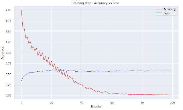
accuracy vs loss curve 3D CNN pytorch


Step 5Display the confusion matrix 

Code :  

 predictionlist=[]
for i in range(len(outputs)):
    p = int(torch.argmax(outputs[i]))
    predictionlist.append(p)
labels1=labels.argmax(-1).tolist()
labels1= [str(x) for x in labels1]
predictionlist= [str(x) for x in predictionlist]
labelsLIST = ['0','1', '2','3', '4','5', '6','7', '8','9']
cm = confusion_matrix(labels1, predictionlist, labels=labelsLIST)
ConfusionMatrixDisplay(cm).plot()
#   ******************** color of confusion matrix 


ax= plt.subplot()
sns.heatmap(cm, annot=True, ax = ax, cmap=plt.cm.Blues); #annot=True to annotate cells

# labels, title and ticks
ax.set_xlabel('Predicted labels');ax.set_ylabel('True labels') 
ax.set_title('Confusion Matrix'); 
ax.xaxis.set_ticklabels( ['0','1', '2','3', '4','5', '6','7', '8','9']); ax.yaxis.set_ticklabels(['0','1', '2','3', '4','5', '6','7', '8','9'])
plt.rcParams['figure.figsize'] = (8, 7)
plt.show()

Confusion matrix 3D CNN Pytorch

Conclusion 

  • 3D CNN follows the same principle as 2D CNN.
  • 3D CNN uses 3D convolution layers to analyze three-dimensional images, allowing for a more sophisticated computing process (a lot of memory space and execution time).
  • Because 3D pictures contain more detail than 2D images, CNN 3D is more prone to overfitting.

Wednesday, February 24, 2021

Densely Connected Networks (DenseNet)


Densely Connected Networks (DenseNet)


Densely Connected Network (DenseNet) is a convolution neural network (CNN) architecture established by Huang in 2017. This model has proven its outperformance in the image classification task compared to ConvNet, ALexNet, and ResNet.

Densely Connected Network (DenseNet) showed significant improvements in comparison with previous deep learning architectures using different datasets such as CIFAR-10, CIFAR-100, SVHN, and ImageNet

DenseNet architecture

DenseNet architecture
DenseNet is formed of blocks in which each layer is connected to all the previous layers. It is characterized by:

The links between all the layers and feature reuse

As seen in the figure below, each layer receives as input all the results of the preceding layers (using concatenation in the forward propagation). We assume that we have N layers the number of connections is N(N+1)/2.

Features concatenation

The diversified features

Thanks to the links between all the layers, this architecture has the advantage of having various features instead of the feature correlated (as in ResNet).

The limited number of parameters

At each step, the input size is equal to l×k and the output size is equal to k (where k is a very small growth rate). In the bottleneck layers batch norm, ReLU and Conv1x1 are used to reduce complexity and size.

The ability to reduce the problem of vanishing-gradient

This problem consists in a bad definition of the hyper-parameters (e.g. weight, bias), this has the consequence that the ANN does not learn or takes a lot of time to learn.

Tuesday, February 23, 2021

Convolution Neural Network (CNN) architectures: overview

Convolutional Neural Network architectures: overview


 In the 1980s, Yann leCun proposed a convolutional neural network, also called ConvNet or CNN, he used it for the first time with the backpropagation algorithm for the training of handwritten recognition of digits problem in 1989.

Convolutional Neural Network is the most commonly used deep learning architecture for image recognition. It is based on a mathematical operation that helps to extract features from images (convolution operation).

There are different ConvNet architectures such as DenseNet, ResNet, AlexNet, VGGNet, LeNet, U-Net, etc.

Deep Learning Models

LeNet

LeNet is proposed by Yann leCun in 1998, it consists of convolutional layers, pooling layers, and fully connected layers. Before transmitting data to a fully connected layer, a flattening process is applied.

Advantages
  • Easy to understand and use,
  • It works well with the problem of character recognition images.
Disadvantages
  • Low performance because it is not very deep,
  • It is especially proposed to deal with the problem of optical character recognition (OCR), therefore low performance with color images.

AlexNet

It is created by Alex Krizhevsky in 2012 to solve the problem of image classification. It’s deeper than LeNet, it has 60 million parameters. AlexNet8 (with eight layers) consists of five convolutional layers and three fully connected layers (two fully connected hidden layers and one fully connected output layer). After the convolutional layer, Max-pooling with a stride equal to 2 is applied. The output values are flattened for transmission to fully connected layers. AlexeNet used the ReLU activation function.

Advantages
  • It contains several hidden layers which makes it perform better than LeNet for processing color images,
  • Allows the use of multiple GPUs,
  • Helps to avoid overfitting problem by using the overlapping pooling,
  • The dropout layer (parameter = 0.5) that alleviates the overfitting problem is used.
Disadvantages
  • It is not able to solve the problem of the vanishing gradient, because the initialization of the weights is based on the normal distribution,
  • Compared to VGGnet and DensNet, AlexNet is shallower,
  • It uses 5 * 5 convolutional filters while 3 * 3 filters are more efficient.

VGG

VGG is proposed in 2014 by the Visual Geometry Group (VGG), it consists of convolutional layers, pooling layers, and fully connected layers. It is built in the form of blocks which becomes widely used in networks proposed after VGG like ResNet and DenseNet. This architecture is the first which exploited the ILSVR2014 in the classification task. There are Different versions of VGG such as VGG11, VGG16 and VGG19.

Advantages
  • It’s deeper and faster than AlexNet,
  • It uses smaller size kernels (3X3 Kernels),
  • Small size kernels and a large number of layers allow it to learn more complex features.
Disadvantages
  • Take a lot of time in the training stage from scratch,
  • This model is not able to solve the vanishing gradient problem.

ResNet

The addition of hidden layers increases the efficiency of such a model, the major problem with very deep models is the overfitting problem. ResNet aims to deal with complex tasks and solving overfitting and vanishing gradient problems.

Advantages
  • Model of great depth, which allows it to solve complex tasks,
  • Greater precision achieved in various tasks,
  • Faster training time,
  • Ability to overcome the overfitting and vanishing gradient problems.
Disadvantages
  • Take a lot of time in the training stage from scratch,
  • A large number of parameters.

DenseNet

Densely Connected networks (DenseNet) is proposed by Huang in 2017, it consists of convolutional layers, pooling layers, dense blocks, and transition layers. In DenseNet each layer is directly connected with all other layers. It is characterized by feature reuse and diversified features (thanks to the concatenation of features).

Advantages
  • A limited number of parameters,
  • Ability to reduce the problem of vanishing-gradient,
  • Diversified features: thanks to the links between all the layers,
  • Feature reuse,
  • Model of great depth, which allows it to solve complex tasks.
Disadvantages
  • A large number of connections between layers make networks more prone to overfitting problem,
  • DenseNet uses multiple memory spaces as it concatenates all features.

Conclusions

  • Over the years, various architectures have been developed to remedy the problems faced, such as the problem of overfitting, vanishing gradient, etc.,
  • The new models are deeper and more efficient in terms of execution time and treatment of complex tasks,
  • The new models retain the thematic blocks and the links between the layers.

Monday, February 22, 2021

Convolution Neural Network (with Use Case - Pytorch)

convolutional neural networks,convolutional neural network,neural network,convolutional neural network explained,neural networks,convolutional neural network tutorial,convolution neural network,convolutional network,convolutional neural network tensorflow,introduction to convolutional neural networks,artificial neural network,what is convolutional neural network,convolutional neural network example


Artificial Intelligence (AI) enables machines to think and adapt to unexpected circumstances.

Machine learning (ML) is a branch of artificial intelligence that intersects math and statistics to produce an experience-based model. The model is constructed by learning from previous data, allowing it to respond to situations never seen before (without being explicitly programmed).


machine learning,deep learning,ai vs machine learning vs deep learning,machine learning vs deep learning,neural network,machine learning vs deep learning vs artificial intelligence,neural networks,deep learning vs machine learning,artificial intelligence vs machine learning,artificial intelligence vs machine learning vs deep learning,deep learning vs neural networks,machine learning vs artificial intelligence,convolutional neural network,artificial neural network
AI vs Machine Learning vs Neural Network vs Deep Learning vs convolution neural network

Deep learning is a subfield of a neural network that is made up of a set of neurons. It is a neural network that contains more than one hidden layer. The additional layers give it the ability to extract high-level features, so it can solve many computer vision problems like image classification.


deep learning,neural networks,neural network,machine learning,neural network tutorial,deep learning vs neural networks,neural networks and deep learning,what is a neural network,neural networks for machine learning,neural network explained,artificial neural network,what is neural network,convolutional neural network,introduction to neural networks,neural network in deep learning,what is deep learning,deep learning neural networks
Neural Network Vs Deep Learning
The simple neural network is made up of three layers, the first layer which is called the input layer, the second layer (hidden layer), and the last layer which is also the output layer. Deep learning is a type of neural network that has numerous hidden layers and can do more complex tasks including object recognition, semantic segmentation, image classification, and so on. The several hidden layers allow for the extraction of semantic features from images.

Recurrent Neural Networks (RNN), Autoencoders, and Convolution Neural Networks (CNN) are examples of deep learning architectures. In computer vision, CNN remains the crux of deep learning algorithms.

Convolution Neural Network

The Convolution Neural Network (CNN or ConvNet) is a deep learning architecture used to detect and recognize objects. CNN starts by filtering and extracting features from images in order to recognize them, and then it uses a down-sampling function to reduce the number of features collected. After that, an activation function will calculate the output. In the subsections that follow, we'll go through the principles of CNN.

Example: image classification using ConvNet:

Image classification

Convolution Neural Network architecture

A convolution Neural Network built to process digital images consists of convolution layers for feature extraction, pooling layers for downsampling feature maps (as seen in the accompanying figure), and a fully connected layer to create the appropriate outputs.

convolutional neural network,convolutional neural networks,convolutional neural network explained,neural network,neural networks,convolution neural network,artificial neural network,convolutional network,convolutional,neural network architectures,convolutional neural network algorithm
Convolution Neural Network architecture

Convolution layer

To acquire the features of a digital image, the convolution layer uses a mathematical operation known as convolution. The kernels and adjacent pixels must be exploited in order to determine the new pixel value, as seen in the following picture.


convolutional neural network,convolutional neural networks,convolutional,convolutional layer,convolutional neural network explained,convolutional network,convolutional neural network tutorial,graph convolutional network,convolutional neural network python,convolutional neural network tensorflow,convolutional nets,pooling layer in a convolution neural network,convolutional networks,convolutional nerual network,graph convolutional networks
Convolutional layer
Where p is the padding and S is stride.

  • Padding: is used to reduce the information loss by inserting zeros around the image margin as indicated in the following figure.
    The pixel in the corner can only be covered once without applying padding (p=0), but the middle pixel will be covered more than once.
padding,convolutional neural network,convolutional neural networks,padding in cnn,convolutional layer,padding convolutional neural network,convolutional neural network padding,pooling layer convolutional neural network,convolutional network,convolution padding,convolution stride padding,convolutional neural network tutorial,convolutional filter,convolutional calculation,convolutional networks,keras conv2d padding,filter in convolutional neural network
Padding

  • Stride: it represents the step (jump) used during the convolution operation.

convolutional neural network,stride,convolutional neural networks,convolutional layer,stride convolutional neural network,convolutional neural network tutorial,stride in convolutional neural network,convolutional neural network explained,convolutional network,convolution stride,convolutional neural network python,what is convolutional neural network,strided convolution,strided convolutions,convolution stride padding,convolutional
Stride
The output size of each convolution layer is calculated according to the following formula.
CNN formula

Activation functions

The activation function is called also the transfer function, it is a mathematical function that is used for determining the desired output of a neural network. It is basically divided into linear (or identity) and nonlinear activation functions. With linear activation functions, it is not possible to use the backpropagation algorithm (the derivative of a linear function is a constant), thus not allowing any relation with the input data. Indeed, it makes the neural network with several hidden layers work as a neural network with only one hidden layer since the linear aggregation of linear functions gives a linear function. Whereas the nonlinear functions go beyond these limits, it consists in stacking the hidden layers of neural networks. There are several nonlinear functions namely sigmoid, ReLU (Rectified Linear Unit), and softmax.
activation functions formula


Pooling layer

It is made up of a down-sampling operation that summarizes the feature map. A well-defined operation, such as MAX or AVG, is used to accomplish the pooling action. It is used to decrease the amount of parameters and computations in the network by following a predetermined stride.

  • Max pooling: It entails choosing the maximum value from the candidate values.
Max-pooling
Max-pooling

  • AVG-pooling: is to calculate the average of the candidate values.
AVG-pooling
AVG-pooling

  • Min-pooling: It entails choosing the manimum value from the candidate values.
Min-pooling
Min-pooling

Fully-connected layer

A vector of size C is returned after using the fully connected layer, where C is the number of classes. Each vector element represents the likelihood that the input image will fall into a specific category.

Use Case

To understand all of the theoretical information in the previous parts, we will implement a CNN step by step.
This section will guide you through the steps of developing a Medical MNIST classifier.

DataSet 

We will utilize the Medical MNIST dataset in this section, which can be downloaded from the Kaggle website. It contains a variety of medical images divided into six classes (AbdomenCT, BreastMRI, CXR, ChestCT, Hand, HeadCT).

Implementation

1. Importing the libraries

import numpy as np
import os
import matplotlib.pyplot as plt
import torch
from tqdm.auto import tqdm
from torch.autograd import Variable
import torch.nn as nn
import torch.nn.functional as F
from torch.optim import *
from sklearn.metrics import confusion_matrix
from sklearn.metrics import ConfusionMatrixDisplay
import seaborn as sns
# for creating validation set
from sklearn.model_selection import train_test_split
2. Read Data
The path to the dataset folder should be specified in the path variable.

  data=[]
labels=[]
Path='path / path / path '
for dirN, _, fileN in os.walk(Path):
    for filename in fileN:
        path=os.path.join(dirN, filename)
        img = np.array(image.imread(path)) 
        data.append(img)
        if "AbdomenCT" in path: 
            labels.append(0)
        elif "BreastMRI" in path: 
            labels.append(1)
        elif "CXR" in path: 
            labels.append(2)
        elif "ChestCT" in path: 
            labels.append(3)
        elif "Hand" in path: 
            labels.append(4)
        elif "HeadCT" in path: 
            labels.append(5)
  

  data= np.array(data)
print("Data :         ", np.array(data).shape)
print("Labels  :      ", len(labels))

pytorch,pytorch cnn,pytorch cnn tutorial,pytorch course,pytorch tutorial,cnn using pytorch,cnn pytorch,cnn en pytorch,code ann pytorch,tutorial pytorch,cnn useing pytorch,pytorch cnn example,tutorial de pytorch,pytorch sequential,coding pytorch model,red neuronal en pytorch,pytorch with brain tumor,pytorch computer vision,how to code a cnn in pytorch,convolutional ann pytorch,image classification pytorch,how to implement pytorch model

3.Prepare the data


  def one_hit_data (target): 
    # Convert to torch Tensor
    target_tensor = torch.as_tensor(target)
    # Create one-hot encodings of labels
    one_hot = torch.nn.functional.one_hot(target_tensor, num_classes=6)
    return(one_hot)


labels= one_hit_data (labels)
  

4. Create  the Accuracy Function 


  def accuracyFUNCTION (predicted, targets):          
    c=0
    for i in range(len(targets)):
        if (predicted[i] == targets[i]):
            c+=1
    accuracy =  c / float(len(targets))
    print('accuracy   = ', c ,'/', len(targets))
    return(accuracy)


5. Create a 2D CNN  for Medical Mnist Classification


  # Create a 2D convolutional neural network model for image classification
class CNN_classification_medical (nn.Module):
    def __init__(self):
        super(CNN_classification_medical, self).__init__()
        self.model= nn.Sequential(
        
        #Conv layer 1    
        nn.Conv2d(1, 32, kernel_size=(3, 3), padding=0),
        nn.ReLU(),
        nn.MaxPool2d((2, 2)),   
        
        #Conv layer 2  
        nn.Conv2d(32, 64, kernel_size=(3, 3), padding=0),
        nn.ReLU(),
        nn.MaxPool2d((2, 2)),
               
        #Flatten
        nn.Flatten(),  
        #Linear 1
        nn.Linear(12544, 64), 
        #Relu
        nn.ReLU(),
        #BatchNorm1d
        nn.BatchNorm1d(64),
        #Dropout
        nn.Dropout(p=0.15),
        #Linear 2
        nn.Linear(64, num_classes)
        )
    
    def forward(self, x):
        # Set 1
        out = self.model(x)
        return out
  

6. Split the data into two parts (training set (60%) and test set (20%))


  X_train, X_test, y_train, y_test = train_test_split(data,labels, train_size=0.60)
  

7. Convert the arrays torch tensors


X_train=torch.as_tensor(X_train)
X_test=torch.as_tensor(X_test)
y_train=torch.as_tensor(y_train)
y_test=torch.as_tensor(y_test)
   

8. The training step


batch_size = 200    
# Pytorch train and test sets
train = torch.utils.data.TensorDataset(X_train.float(),y_train.long())
test = torch.utils.data.TensorDataset(X_test.float(),y_test.long())
# data loader with pytorch
train_loader = torch.utils.data.DataLoader(train, batch_size = batch_size, shuffle = False)
test_loader = torch.utils.data.DataLoader(test, batch_size = batch_size, shuffle = False)
# we have 6 classes 
num_classes = 6


print('X_train   :   shape:', X_train.shape, '          type:', type(X_train))
print('y_train   :   shape:', y_train.shape, '                     type:', type(y_train))
print('X_test    :   shape:', X_test.shape, '           type:', type(X_test))
print('y_test    :   shape:', y_test.shape, '                      type:', type(y_test))
   

medical mnist, pytorch,mnist,pytorch course,pytorch tutorial,pytorch mnist,pytorch image classification,mnist dataset python,tutorial pytorch,tutorial de pytorch,pytorch sequential,pytorch dataloader,dataloader pytorch,torch,image classification pytorch,pytorch project,pytorch prepare dataset,pytorch projects,dataloader pytorch images


  # The number of epochs (here the number of iterations is = 5000 / we have 50 epochs a batch size is 100 / 50*100=5000) 
num_epochs = 5
# 3D model 
model = CNN_classification_medical()
#You can use the GPU by typing: model.cuda()
print(model)
# Loss function : Cross Entropy
error = nn.CrossEntropyLoss()
# Learning rate : learning_r = 0.001 
learning_r = 0.01
# SGD optimizer
optimizer = torch.optim.SGD(model.parameters(), lr=learning_r)
#***********************************************************************training***********************************
itr = 0
loss_list = []
iteration_list = []
accuracy_list = []
for epoch in range(num_epochs):
    for i, (images, labels) in tqdm(enumerate(train_loader)):
        #print('images.size(0)  11111      ',images.size(0))
        train = Variable(images.view(images.size(0),1,64,64))
        labels = Variable(labels)
        #  zero_grad : Clear gradients
        optimizer.zero_grad()
        # Forward propagation / CNN_classification_model
        outputs = model(train)
        # Calculate loss value / using cross entropy function 
        labels= labels.argmax(-1)
        loss = error(outputs, labels)
        loss.backward()
        # Update parameters using SGD optimizer 
        optimizer.step()
        
        #calculate the accuracy using test data
        itr += 1
        if itr % 100 == 0:
            # Prepare a list of correct results and a list of anticipated results.     
            listLabels=[]
            listpredicted=[]
            # test_loader
            for images, labels in test_loader:
​
                test = Variable(images.view(images.size(0),1,64,64))
                #print('images.size(0)  22222             ',images.size(0))
                # Forward propagation
                outputs = model(test)
​
                # Get predictions from the maximum value
                predicted = torch.max(outputs.data, 1)[1]
                
                # used to convert the output to binary variables
                predicted= one_hit_data (predicted) 
                # Create a list of predicted data
                predlist=[]
                for i in range(len(predicted)):
                    p = int(torch.argmax(predicted[i]))
                    predlist.append(p)
​
                
                listLabels+=(labels.argmax(-1).tolist())
                listpredicted+=(predlist)
​
                
                # calculate Accuracy
            accuracy= accuracyFUNCTION(listpredicted, listLabels)
            print('Iteration: {}  Loss: {}  Accuracy: {} %'.format(itr, loss.data, accuracy))
​
            # store loss and accuracy. They'll be required to print the curve.
            loss_list.append(loss.data)
            accuracy_list.append(accuracy)
​
 

pytorch,pytorch image classification,image classification using resnet model in pytorch,cnn model for image classification,image classification in pytorch,image classification pytorch,image classification,handwritten digit classification,increase accuracy of model on small dataset,pytorch course,pytorch tutorial,pytorch mnist,image classification tutorial,text classification,multi label text classification,cnn image classification


9. Display The Confusion Matrix 

  
  predictionlist=[]
for i in range(len(outputs)):
    p = int(torch.argmax(outputs[i]))
    predictionlist.append(p)
labels1=labels.tolist()


labels1= [str(x) for x in labels1]
predictionlist= [str(x) for x in predictionlist]
labelsLIST = ['0','1', '2','3', '4','5']
cm = confusion_matrix(labels1, predictionlist, labels=labelsLIST)
ConfusionMatrixDisplay(cm).plot()
#   ******************** color of confusion matrix 


ax= plt.subplot()
sns.heatmap(cm, annot=True, ax = ax, cmap=plt.cm.Blues); #annot=True to annotate cells

# labels, title and ticks
ax.set_xlabel('Predicted labels');ax.set_ylabel('True labels') 
ax.set_title('Confusion Matrix'); 
ax.xaxis.set_ticklabels( ['AbdomenCT  ','BreastMRI', 'CXR','ChestCT', 'Hand','HeadCT']); ax.yaxis.set_ticklabels(['AbdomenCT   ','BreastMRI', 'CXR','ChestCT', 'Hand','HeadCT'])
plt.rcParams['figure.figsize'] = (9, 8)
plt.show()
  
confusion matrix,image classification,confusion matrix vs classification report,confusion matrix for multiclass classification,pytorch,sklearn confusion matrix,cnn model for image classification,confusion matrix multi-class,confusion matrix python,what is confusion matrix,confusion matrix in python,plot confusion matrix python,pydata confusion matrix,what is a confusion matrix in machine learning,true positive rate confusion matrix


Conclusions

  • CNN is a deep learning architecture that is used to analyse images (for example, image classification and semantic segmentation, etc.),
  •  CNN is built up of convolutional layers that use the convolution operation to extract features. Pooling layers for down-sampling feature maps, and a fully connected layer,
  • There are various operations that can be applied in the pooling layer, such as Max or AVG.